Quantitative (Quant) Trader gemchange_ltd posted a long article on X outlining his complete roadmap for “if I had to start over tomorrow,” from probability theory to stochastic calculus—five math hurdles, 18 months from zero to true entry-level quant trading. The article is adapted and reorganized from his popular post on X, “How I’d Become a Quant If I Had to Start Over Tomorrow,” translated and compiled by Flip.
(Background: A trader who relies solely on analysis of cycles, no commissions, no exposure—just winning strategies.)
(Additional context: Top female crypto trader’s 10,000-word survival notes: Don’t let “get-rich-quick” ruin you.)
Table of Contents
Toggle
- Part I: Probability Theory—The Language of Uncertainty
- Part II: Statistics—Learning to Listen to Data
- Part III: Linear Algebra—The Engine Behind Everything
- Part IV: Calculus & Optimization—The Language of Change
- Part V: Stochastic Calculus—The True Threshold of Quant
- Polymarket
- Quant Trading Career Map: Four Archetypes
- Toolbox & Reading List
- Three Things the Author Wishes He Knew Earlier
Disclaimer: This article does not constitute investment advice. Markets carry risks—do your own research.
Starting with a few numbers: By 2025, top-tier institutions’ fresh Quant annual total compensation ranges from $300K to $500K. AI/ML hiring in finance grows 88% annually. Is there a map for this path?
This article is what the author wishes someone had handed him at the start. The learning route is arranged in “the order you should learn,” with each concept built on the previous—like a video game, you can’t skip levels. But if you really commit, not wasting time on boring YouTube finance intro videos (which are just time sinks), but actually solving problems and hands-on practice—about 18 months, you can go from zero to understanding some fundamentals.
Put aside all the trading knowledge you think you know. Most believe quant trading is stock picking, having opinions on Tesla, or forecasting earnings. It’s not. Quant is math. You’re modeling statistical relationships, pricing inefficiencies, and structural advantages arising from the fact that “markets are run by people who systematically make mistakes.”
Part I: Probability—The Language of Uncertainty
Everything in quantitative finance boils down to one question: What’s the win rate? Is it on my side?
That’s probability. If you don’t deeply understand probability, nothing in the rest of this article will make sense.
Conditional Probability: The Quant Mindset
Most think in absolutes: this is true or false. Quant thinks conditionally: given what I know now, what’s the probability this is true?
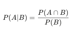
P(A|B) = P(A∩B) / P(B)—Given B has occurred, the probability of A is the probability both A and B happen divided by the probability of B. Sounds simple, but it’s profound. For example, a stock has a 60% chance of rising on any given day—basic probability. But on days with above-average volume, the chance of a rise is 75%. That conditional probability is meaningful; the original 60% is noise.
Bayes’ Theorem: Updating Judgments in Real Time
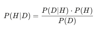
Posterior = (Likelihood of data given hypothesis) × Prior / Total probability of data.
In practice, use Monte Carlo sampling to compute. The logic is the same: Bayes’ theorem lets you update your beliefs instantly when new info arrives. If your model says a stock should be worth $50, but earnings come out 3% above expectations—your posterior probability shifts upward. The fastest, most accurate updates win.
Expected Value & Variance: Your Two Best Friends
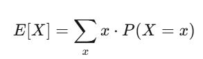
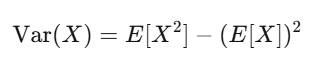
Expected value reflects your confidence; variance measures your risk. If your strategy has positive expected value and you can withstand the swings from variance, you’re likely to profit.
Level 1 Tasks (2 hours daily, 3-4 weeks)
- Read: Blitzstein & Hwang, Introduction to Probability (free PDF from Harvard), do all exercises in chapters 1-6
- Code: Simulate 10,000 coin flips, visualize Law of Large Numbers
- Code: Implement a Bayesian updater—input prior and likelihood, output posterior
import numpy as np
import matplotlib.pyplot as plt

# Law of Large Numbers demonstration
np.random.seed(42)
flips = np.random.choice([0, 1], size=10000, p=[0.5, 0.5])
running_avg = np.cumsum(flips) / np.arange(1, 10001)

plt.figure(figsize=(10, 4))
plt.plot(running_avg, linewidth=0.7)
plt.axhline(y=0.5, color='r', linestyle='--', label='True Probability')
plt.xlabel('Number of Flips')
plt.ylabel('Running Average')
plt.title('Law of Large Numbers Demo')
plt.legend()
plt.savefig('lln.png', dpi=150)
print(f"After 10,000 flips: {running_avg[-1]:.4f} (True: 0.5000)")
Part II: Statistics—Learning to Listen to Data
Once you speak probability, the next skill is extracting signals from data. The first lesson: Most seemingly meaningful findings are just noise.

Hypothesis Testing: Your Noise Filter
Build a model with backtested annual return of 15%. Is it real? Set null hypothesis H₀: “This strategy’s expected return is zero,” compute test statistic, p-value. But beware: testing 1,000 random strategies, pure luck can produce about 50 p-values below 0.05—multiple comparisons problem. Use Bonferroni correction or Benjamini-Hochberg FDR control. Beginners tend to overestimate their discoveries. Accept that most are noise—save yourself money.
Regression Analysis: Decomposing Returns

Linear regression y = Xβ + ε is core in finance. Regress strategy returns against known risk factors; the intercept α is your alpha—excess return unexplained by factors.
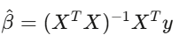
If after controlling for factors, α ≈ 0, your so-called “edge” is just disguised market exposure. Use Newey-West standard errors—financial data have autocorrelation and heteroskedasticity. Ordinary least squares standard errors are like driving with a cracked windshield at high speed.
Maximum Likelihood Estimation (MLE)
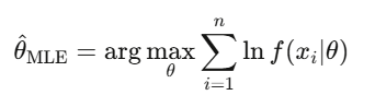
This is how finance calibrates models—fitting GARCH volatility, estimating jump diffusion parameters, aligning option prices with market quotes. When someone says “calibrating” a model, they usually mean MLE.
Level 2 Tasks (4-5 weeks)
- Read: Wasserman, All of Statistics, chapters 1-13
- Download real stock returns (yfinance), test for normality (it fails), fit t-distribution via MLE, compare
- Run Fama-French three-factor regressions on stock portfolios using statsmodels
- Implement permutation tests: shuffle dates 10,000 times, compare permuted vs. actual performance
Part III: Linear Algebra—The Engine of Everything
Linear algebra sounds dull but is the core engine: portfolio construction, PCA, neural networks, covariance estimation, factor models. No matrices, no quant.

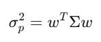
Matrix Thinking
Covariance matrix Σ captures how assets move relative to each other. For 500 stocks, Σ is 500×500 with 125,250 unique entries. Portfolio variance simplifies to w’Σw—central to Markowitz, risk management, everything.
Eigenvalues: The Real Deal
In a universe of 500 stocks, the top 5 eigenvectors explain 70% of total variance. Others are noise. Using eigen-decomposition transforms the world: dimension reduction, basis for factor investing.
Level 3 Tasks (4-6 weeks)
- Watch Gilbert Strang’s MIT 18.06 Linear Algebra course—full, no skipping
- Read: Strang, Introduction to Linear Algebra, do all exercises
- Perform PCA on S&P 500 returns, plot eigenvalue spectrum, identify top 3 components
- Implement Markowitz mean-variance optimization from scratch
import numpy as np
import cvxpy as cp

np.random.seed(42)
n_assets = 10
mu = np.random.uniform(0.04, 0.15, n_assets)
A = np.random.randn(n_assets, n_assets) * 0.1
cov = A @ A.T + np.eye(n_assets) * 0.01

w = cp.Variable(n_assets)
objective = cp.Minimize(cp.quad_form(w, cov))
constraints = [
    mu @ w >= 0.08,   # minimum return
    cp.sum(w) == 1,   # fully invested
    w >= -0.1,        # max 10% short
    w <= 0.3          # max 30% long
]

prob = cp.Problem(objective, constraints)
prob.solve()

ret = mu @ w.value
vol = np.sqrt(w.value @ cov @ w.value)
sharpe = (ret - 0.03) / vol

print(f"Portfolio Return: {ret:.4f}")
print(f"Portfolio Volatility: {vol:.4f}")
print(f"Sharpe Ratio: {sharpe:.4f}")
Part IV: Calculus & Optimization—The Language of Change
Calculus describes change. In finance, everything changes: prices, volatilities, correlations, distributions every second. Calculus models and exploits these changes. Derivatives appear in neural network backpropagation and option Greeks.

Taylor expansions approximate Delta hedging; Gamma hedging adds second-order correction. Itô calculus differs from ordinary calculus because the second-order term (dW_t)^2 ≈ dt doesn’t vanish.
Level 4 Tasks (4-5 weeks)
- Read: Boyd & Vandenberghe, Convex Optimization (free Stanford PDF), chapters 1-5
- Implement gradient descent to minimize Rosenbrock function from scratch
- Use cvxpy to solve a portfolio optimization with transaction costs
Part V: Stochastic Calculus—The Real Quant Threshold
Before learning stochastic calculus, you’re just a data scientist interested in finance. After, you’re a true Quant. It’s about modeling randomness in continuous time, deriving Black-Scholes from first principles, understanding why derivatives markets operate as they do.

Brownian Motion: Formalizing Randomness
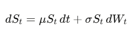
Brownian motion (Wiener process) W_t is a continuous-time random walk. The key insight—and the foundation of everything—is that dW_t’s “size” is √dt, meaning (dW_t)^2 = dt. Sounds technical, but it’s the most critical fact in quant finance.
Itô’s Lemma
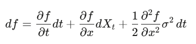
In ordinary calculus, you expand in Taylor series, (dx)^2 is negligible. But if x is a stochastic process, (dW_t)^2 = dt is a first-order term—you can’t ignore it. Itô’s lemma: df = (∂f/∂t + μ∂f/∂x + ½σ²∂²f/∂x²)dt + σ∂f/∂x dW_t. Applying this to option pricing yields Black-Scholes.
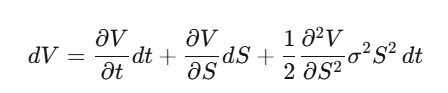
Deriving Black-Scholes from scratch
Step 1: Let V(S,t) be the option price, apply Itô’s lemma.
Step 2: Construct a delta-hedged portfolio Π = V − (∂V/∂S)·S, compute dΠ—dW_t terms cancel perfectly, making the portfolio locally riskless.
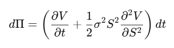
Step 3: A riskless portfolio must grow at the risk-free rate.
Step 4: Rearrange to get the Black-Scholes PDE.
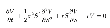
Notice what happens: drift μ disappears. The option price is independent of the stock’s expected return and risk preferences. You can price options under the risk-neutral measure. Truly understanding this is mind-bending.
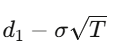
For a European call with strike K and expiry T, the solution is:
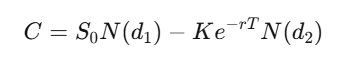
where d_1=
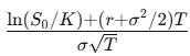
d_2=
Greek Letters
- Delta Δ: How much the option moves per dollar move in underlying
- Gamma Γ: Rate of change of Delta—convexity risk
- Theta Θ: Time decay—usually negative for long positions
- Vega V: Sensitivity to volatility—most derivatives profit here
- Rho ρ: Sensitivity to interest rates
import numpy as np
from scipy.stats import norm

def black_scholes(S, K, T, r, sigma, option_type='call'):
    d1 = (np.log(S/K) + (r + sigma**2/2)*T) / (sigma*np.sqrt(T))
    d2 = d1 - sigma*np.sqrt(T)
    if option_type == 'call':
        return S*norm.cdf(d1) - K*np.exp(-r*T)*norm.cdf(d2)
    else:
        return K*np.exp(-r*T)*norm.cdf(-d2) - S*norm.cdf(-d1)

def monte_carlo_option(S0, K, T, r, sigma, n_sims=500_000):
    Z = np.random.standard_normal(n_sims)
    ST = S0 * np.exp((r - sigma**2/2)*T + sigma*np.sqrt(T)*Z)
    payoffs = np.maximum(ST - K, 0)
    price = np.exp(-r*T) * np.mean(payoffs)
    stderr = np.exp(-r*T) * np.std(payoffs) / np.sqrt(n_sims)
    return price, stderr

S, K, T, r, sigma = 100, 105, 1.0, 0.05, 0.2
bs_price = black_scholes(S, K, T, r, sigma)
mc_price, mc_err = monte_carlo_option(S, K, T, r, sigma)
print(f"Black-Scholes Price: ${bs_price:.4f}")
print(f"Monte Carlo Price: ${mc_price:.4f} ± {mc_err:.4f}")
Level 5 Tasks (6-8 weeks, hardest level)
- Read: Shreve, Stochastic Calculus for Finance II (standard reference)
- Alternative: Arguin, A First Course in Stochastic Calculus (more accessible)
- Derive the stochastic differential of f(S) = ln(S), recover the -σ²/2 drift
- Derive the full Black-Scholes PDE from delta hedging
- Implement Black-Scholes and Monte Carlo from scratch, compare convergence
Polymarket
The most interesting market today, with math connecting all these topics:
Probability, Information Theory, Convex Optimization, Integer Programming.
How LMSR Prices Beliefs
Logarithmic Market Scoring Rule (LMSR)
Invented by Robin Hanson, used for automated prediction markets.
For n outcomes, the cost function is:
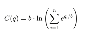
where:
- q_i: outstanding shares of outcome i
- b: liquidity parameter
The price of outcome i is:
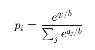
This is essentially a softmax function—the same used in neural network classifiers.
Properties:
- All prices sum to 1
- All prices are in (0,1)
- Market always has prices—providing infinite liquidity
Market Maker’s Max Loss
Limited to: b × ln(n)
Quant Trading Career Map: Four Archetypes
Quant Researcher (QR): Finds patterns in petabyte-scale data, builds predictive models, designs strategies. Requires PhD-level math/statistics/ML or exceptional undergrad talent. At firms like Jane Street, QR has access to thousands of GPUs.
Quant Developer/Engineer (QD): Builds trading platforms, execution engines, real-time data pipelines—making research models tradable. Needs production-grade C++/Rust/Python and low-latency systems.
Quant Trader (QT): Decision-maker, manages capital, controls risk, makes real-time judgments. Highest variance in pay; top years reach eight figures.
Risk Quant: Gatekeeper—model validation, VaR, stress testing, compliance. More stable career path, lower ceiling. Emerging AI/ML roles (using deep learning signals) grow fastest—88% annual hiring increase in 2025.
Salary ranges (top US firms: Jane Street, Citadel, HRT):
- Entry: $300K–$500K+ total package
- Mid-level (3–7 years): $550K–$950K
- Senior (8+ years): $1M–$3M+
- Star traders/PMs: $3M–$30M+
Mid-sized firms (Two Sigma, DE Shaw): entry ~$250K–$350K total. Jane Street’s average compensation in early 2025 hits $1.4M/year.
Interview process: Resume screening → Online test (mental math with Zetamac, target 50+ points, logic puzzles) → Phone interview (probability, gambling games) → Superday (3–5 rounds: trading simulation, coding, whiteboard derivations). Jane Street intentionally makes questions hard—testing how you leverage hints and collaborate. Most interns are CS or Math majors; finance knowledge not required.
Preparation tips: Xinfeng Zhou’s Green Book (quant interview guide, 200+ real questions), QuantGuide.io (quant LeetCode), Brainstellar.
Toolbox & Reading List
Python stack: pandas/polars (Polars 10–50× faster on big data), numpy/scipy, xgboost/lightgbm, pytorch, cvxpy, QuantLib, statsmodels, NautilusTrader/vectorbt.
Free data sources: yfinance, Finnhub (60 requests/min), Alpha Vantage. Mid-tier: Polygon.io ($199/month, <20ms latency). Enterprise: Bloomberg Terminal (~$32,000/year).
Books (in order):
Math fundamentals: Blitzstein & Hwang Probability → Strang Linear Algebra → Wasserman All of Statistics → Boyd & Vandenberghe Convex Optimization → Shreve Stochastic Calculus I & II
Quant finance: Hull Options, Futures, and Other Derivatives → Natenberg Option Volatility & Pricing → López de Prado Advances in Financial Machine Learning → Ernest Chan Quantitative Trading → Zuckerman The Man Who Solved the Market
Interviews: Zhou Green Book → Crack Heard on the Street → Joshi Quant Interview Questions
Competitions: Jane Street Kaggle ($100K prize), WorldQuant BRAIN (over 100K users, buy alpha signals), Citadel Datathon (fast track to full-time)
Three Things the Author Wishes He Knew Earlier
Estimation error is the real enemy. Full Kelly betting, unconstrained Markowitz, ML models with many features—all fail for the same reason: overfitting noise in parameter estimates. Math works perfectly under true parameters, but you never have true parameters. The gap between theory and practice is always estimation error. The best Quant respects this.
Tools are democratized, judgment is not. Anyone can access QuantLib, Polygon.io, PyTorch. Tech is necessary but not sufficient. Advantage lies in unique data, models, execution—more than just better pip installs.
Math is the moat. AI can code, suggest strategies, but only math—deriving why Itô’s lemma has that extra term, proving the martingale property under risk-neutral measure, knowing whether convex relaxations are tight—distinguishes “building advantage” Quant from “borrowing advantage.” Borrowed advantage expires.